
効率化の測定で、私の数字は3回嘘をついた
小規模なMixture of Experts実験で見つかった、結果を誤らせる測定上の欠陥3件の記録です。3件とも、エラーを出さず、もっともらしい数値を返していました。そのまま報告していれば、過大な主張になっていたものです。
小規模 MoE 実験における測定欠陥の記録
この文書について
規模:最大 500 万パラメータの Transformer、合成分類タスク、CPU のみ。 実運用の言語モデルとは 3〜5 桁の隔たりがあります。ここに出てくる削減率を、 設備規模に換算することはできません。
新規性:実装した機構(専門家への専門領域強制、トークンごとの可変配分、 プロンプト単位の経路振り分け)は、いずれも既存手法の再実装です。新しい アルゴリズムの提案ではありません(詳細は「関連研究」の章)。
それでも書く理由:検証の過程で、結果を誤らせる測定上の欠陥を 3 件 発見しました。3 件とも、
- エラーを出さなかった
- もっともらしい数値を返していた
- そのまま報告すれば、過大な主張になっていた
そして 3 件とも、この研究に固有ではありません。適応的計算を測る人、 ハイパーパラメータを振る人、合成ベンチマークを作る人が、同じ形で踏みうるものです。
削減率は転用できませんが、検算の方法は転用できます。 それがこの文書の主題です。
1. 何を作ったか
「回答精度を落とさずに、1トークンあたりの計算量を削減できるか」を検証するため、 条件付き計算(Mixture of Experts)を用いた小規模 Transformer を実装しました。
タスクは合成分類(8クラス、100ユーザー、語彙128、系列長16)。全サンプルの約35%は 曖昧サンプルで、入力トークンだけでは正解が決まらず、ユーザーの嗜好によってのみ 決定されます。この設計により「個別化が効いているか」が測定可能になります。
以降、3 件の欠陥を順に記述します。結果は最後にあります(欠陥の説明が先でないと、 なぜその数字が信用できるのかが分からないためです)。
2. 欠陥1:訓練データに暗記の抜け道があった
症状
訓練損失         →  0.0000
曖昧サンプルの
テスト精度       →  0.125(=まぐれ当たり)
訓練データは完璧に適合できているのに、テストではまぐれ当たり。
さらに悪いことに、全条件がまぐれ当たりで並びました。対照モデル(ユーザー埋め込みを 出力層に直結した上限モデル)を含めて。
c(u) のみ        0.1516 ± 0.0350
c(u, x) τ=0.2    0.1526 ± 0.0298
c(u, x) τ=0.4    0.1657 ± 0.0425
対照             0.1259 ± 0.0265   ← 上限モデルも動いていない
まぐれ当たり      0.1250
p 値: 0.60 / 0.61 / 0.62
原因
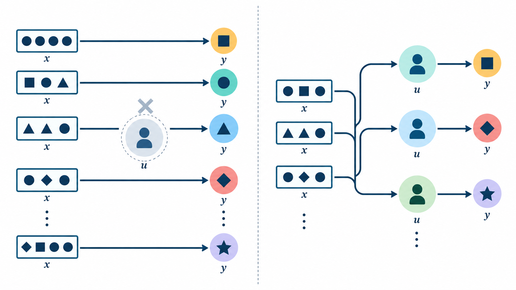
曖昧サンプルのトークン列が、1 件ごとに固有でした。
訓練中の曖昧サンプル      467 件
固有のトークン列          467 種
ラベルが衝突する入力        0 件
衝突がゼロということは、「このトークン列=この答え」という対応を丸暗記すれば 訓練損失が 0 になるということです。ユーザー埋め込みを参照する必要が一度も生じない。 そして丸暗記は未知のサンプルに転移しないので、テストではまぐれ当たりに戻る。
タスクの説明文には「曖昧サンプルはユーザーしか解けない」と書いてありました。 実際には、訓練中に限りトークン列そのものが答えになっていました。
検証
「そもそも解けるタスクなのか」を確認しました。ユーザー埋め込みから主要トピックを 線形プローブで予測できるかを測定:
学習済みユーザー   1.0000
未知のユーザー     0.8500
まぐれ当たり       0.1250
タスクは解けます。 抜け道のほうが安かっただけでした。
修正
曖昧入力を共有プール(64種)から抽出するよう変更。同じ入力が、正解の異なる ユーザーに提示されます。
修正前  固有 467 種、ラベル衝突 0 件
修正後  固有  64 種、ラベル衝突 64 件(全入力)
丸暗記が自己矛盾を起こすので、ユーザー埋め込みを見るしかなくなります。
効果
対照モデルの曖昧サンプル精度:
epoch  1   0.118
epoch 20   0.355
epoch 30   0.509   ← まぐれ当たりの 4 倍
ここで初めて実験に検出力が生まれました。 修正前は、対照が動かない状態で 「ルーティングは効かない」と結論しかけていました。上限が動かない実験に、 何かを否定する力はありません。
一般化できる形
合成ベンチマークで「難しいケース」を作るとき、
その入力が1件ずつ固有だと、暗記経路が開く。

確認方法: 訓練データ内で、同じ入力に異なる正解が付いている件数を数える。
         ゼロなら、その「難しさ」は訓練中には存在しない。
3. 欠陥2:モデルの重みが seed されていなかった
症状
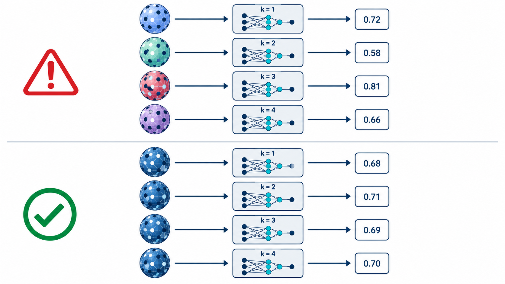
同一の設定・同一の seed で 2 回実行し、結果が違いました。
1回目:  k=1 0.2182   k=2 0.5364   k=3 0.6182
2回目:  k=1 0.2455   k=2 0.3727   k=3 0.5818
                         ↑ 0.16 の差
原因
seed_everything が実験ランナーからのみ呼ばれていました。研究用モジュールが
モデルを直接構築する経路では、PyTorch の重み初期化が未 seed でした。
データセットは seed されていた(NumPy 経由)ので、部分的には再現していました。 それが発覚を遅らせました。
影響
これが深刻なのは、スイープの前提を壊すからです。
意図:  k だけを変えて比較する
実際:  k と初期重みを同時に変えていた
sweep_parameter の docstring に「同じ seed、同じ初期重み」と私が書いていましたが、
事実ではありませんでした。
この欠陥の下で、k=3 に極大が観測されていました。修正後、5 シードで測り直すと:
k   精度              曖昧サンプル
1   0.7033 ± 0.0375   0.1840 ± 0.0570
2   0.7853 ± 0.0230   0.4023 ± 0.0642
3   0.8247 ± 0.0329   0.5187 ± 0.1182
4   0.8347 ± 0.0405   0.5490 ± 0.1212

k=3 対 k=4: p = 0.700
k=3 が最良だったシード: 5 回中 1 回
単調増加で、極大は存在しませんでした。 k=3 の山は欠陥が作った幻です。
修正
seed_everything をモデル構築時に呼ぶよう移動。config.seed が、どこでモデルを
作っても仕様通りの意味を持つようにしました。
テスト: - 同一設定で 2 回作った重みが一致する - 異なる seed では一致しない - スイープの各候補が同一の初期重みを持つ
一般化できる形
確認方法: 同じ設定でモデルを2回構築し、最初のパラメータテンソルを比較する。
         一致しなければ、あなたのスイープは2つの変数を同時に動かしている。
4. 欠陥3:可変計算モデルの FLOPs を 1 サンプルで測っていた
症状
平均 k が異なる 3 構成が、完全に同一の FLOPs を報告しました。
構成              平均 k    実測 FLOPs
cascade cover 0.7  1.83     1,829,888
cascade cover 0.9  2.58     1,829,888   ← 同値
固定 k=1           1.00     1,829,888   ← これとも同値
平均 k が 2.58 と 1.00 で、消費が 2 倍以上違うはずの構成が、同じ値を返す。
原因
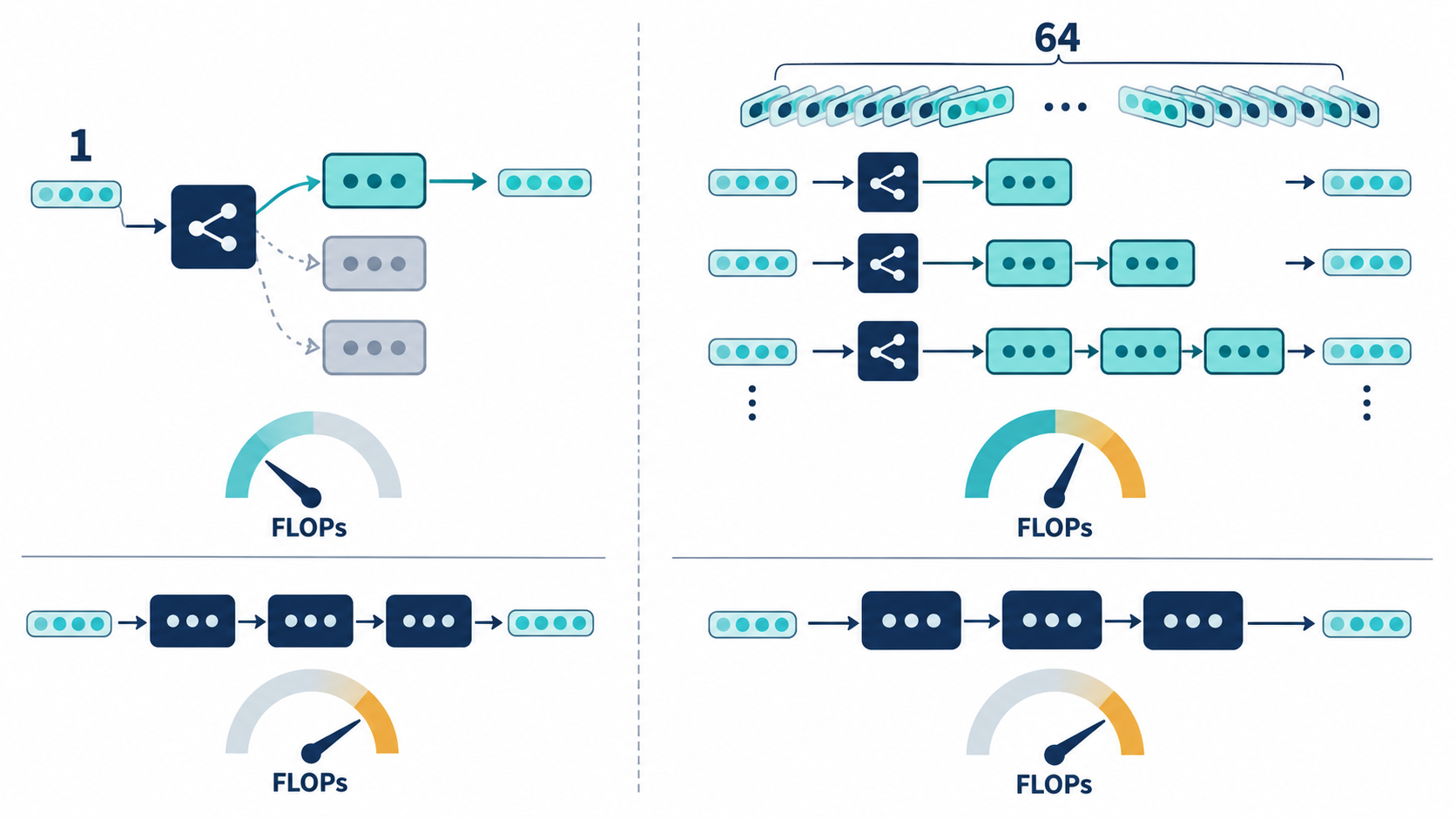
measure_flops_per_sequence が、1 サンプルだけで測定していました。
固定計算のモデルなら、1 サンプルで正確です。しかしトークンごとに消費が変わる モデルでは、1 サンプルは「そのサンプルの値」であって「モデルの値」ではありません。
測定に使われたサンプルがたまたま容易で、全構成が k=1 に収束していました。
影響
修正前の値をそのまま使えば、3 構成すべてを「44.6% 削減」と報告していました。 実際の値は 35.4% / 26.5% / 44.6% です。
そしてこの数字は、半導体供給の議論に持ち込まれる予定でした。
修正
64 サンプルの平均に変更。
テスト: - 専門家を多く使う構成は、必ず高い FLOPs を報告する(これが見えない測定では 削減も見えない) - 密なモデルは、サンプル数を変えても同じ値を返す
一般化できる形
適応的計算・MoE・早期終了など、入力によって計算量が変わるモデルでは、
FLOPs を 1 サンプルで測ってはいけない。

確認方法: 設定を変えた2つのモデルで測り、消費が違うはずなのに
         同じ値が出たら、測定が入力に依存している。
5. 3 件に共通する兆候
3 件とも、次の性質を持っていました。
エラーを出さない
もっともらしい数値を返す
数値だけ見ても異常が分からない
唯一の検出手段は、機構が許すより正確に数値が一致していたことでした。
欠陥1  全条件がまぐれ当たり 0.125 付近で並んだ
欠陥2  同一条件の2回の実行が一致しなかった(逆パターン)
欠陥3  平均 k が違う3構成の FLOPs が完全に一致した
「結果が綺麗すぎる」「一致しすぎる」は、安心材料ではなく症状として扱うべきものだと 考えます。
6. 結果(事例として)
3 件の修正を経た後の数値です。5 シード(42, 123, 456, 789, 2026)。
6.1 対照の選び方
初期の比較では対照を「ユーザー情報を持たない密なモデル」としていましたが、これは 疎化の効果と個別化の効果を混同します。全条件が同一の情報を持つ状態で計算量のみを 比較するため、対照を 密なモデル + ユーザー埋め込み直結 に変更しました。
6.2 精度と計算量
| 構成 | 精度 | 対照差 | p | 実測FLOPs | 削減率 |
|---|---|---|---|---|---|
| 対照(密 + z_u) | 0.8360 ± 0.0148 | 基準 | — | 3,305,472 | 0.0% |
| 表札 k=1 | 0.7067 ± 0.0292 | −0.1293 | 0.000 | 1,829,888 | 44.6% |
| 表札 k=2 | 0.7987 ± 0.0441 | −0.0373 | 0.134 | 2,354,176 | 28.8% |
| 表札 k=3 | 0.8273 ± 0.0437 | −0.0087 | 0.692 | 2,878,464 | 12.9% |
| カスケード cover 0.7 | 0.8147 ± 0.0514 | −0.0213 | 0.416 | 2,136,320 | 35.4% |
| カスケード cover 0.9 | 0.8433 ± 0.0376 | +0.0073 | 0.701 | 2,428,570 | 26.5% |
カスケード cover 0.9 のみ、差の点推定が正です。
ブートストラップ 95% 信頼区間  [−0.024, +0.039]
効果量 Cohen's d              +0.256(小)
シード別                       +0.0367 / −0.0167 / +0.0233 / −0.0267 / +0.0200
信頼区間はゼロをまたぎます。「劣化していない」とは言えますが、「改善した」とは
言えません。 また p > 0.05 は差がないことの証明ではなく、n=5 では 0.03 程度の
実在する劣化を見逃します。
6.3 可変配分は固定配分に優越する
| 構成 | 精度 | 削減率 |
|---|---|---|
| 固定 k=3 | 0.8273 | 12.9% |
| カスケード cover 0.9 | 0.8433 | 26.5% |
同一精度帯で削減率が 2 倍。全トークンに同額を配分することの非効率が定量化されました。
6.4 メモリは逆方向に動く
| 指標 | 対照比 |
|---|---|
| 活性パラメータ(1トークンの演算) | −20.1% |
| 総パラメータ(常駐メモリ) | +63.6% |
専門家 8 体のうち走るのが 1〜3 体でも、どれが選ばれるか事前に分からないため全体を 常駐させる必要があります。条件付き計算は演算とメモリを交換します。
6.5 この手法の天井
FLOPs の内訳(対照モデル、系列長 16):
feed-forward(この手法の対象)  63.4%
attention                     35.7%
その他                          0.9%
FFN を完全にゼロにしても、上限は 63.4% 削減です。attention には手が届きません。 達成した 26.5% は、この天井の 41.8% に相当します。
そして attention は系列長の 2 乗で増えるため、長文脈では天井がさらに下がります。 この方向は、努力ではなく構造によって上限が決まっています。
7. 「効率化」は 3 つの独立な軸である
| 技術 | メモリ | 演算量 | 実時間 |
|---|---|---|---|
| MoE カスケード | 増(+63.6%) | 減(−26.5%) | 未測定 |
| int8 量子化 | 減(−42.0%) | 減 | 増(+33%) |
int8 量子化の実測ログ:
0.44 MB → 0.26 MB(42.0% 削減)、5 モジュール置換
レイテンシ 0.90ms → 1.20ms(0.75倍)
理由: このテンソルサイズでは、量子化・逆量子化のオーバーヘッドが
      節約した演算量を上回る
メモリが 42% 減り、実時間が 33% 悪化しました。 大規模テンソルでは逆転すると 考えられますが、それは本実験で確認したものではありません。
「効率化した」という一語では、どの軸が良くなり、どの軸が悪くなったかが失われます。
8. 関連研究
本実験で実装した機構は、いずれも新規ではありません。 該当する既存分野を示します。
| 実装 | 対応する既存手法 |
|---|---|
| 表札(専門家への専門領域強制) | 教師ありルーティング、補助損失付き MoE |
| カスケード(トークンごとの可変 k) | 適応的計算、動的専門家配分 |
| プロンプト単位の経路振り分け | モデルカスケード、クエリルーティング |
| c(u, x) による信頼度ゲート | 条件付き計算一般 |
条件付き計算・MoE は確立した研究分野であり、大規模言語モデルでの実装例も複数存在します。 本実験はそれらを小規模に再実装し、測定の妥当性を検証したものです。
新規性を主張しているのは、機構ではなく測定欠陥の記録のみです。そしてそれも、 「これらの欠陥が未知である」という主張ではなく、「実際に踏んだ記録として残す」 という性質のものです。
9. 限界
- 規模 — 最大 500 万パラメータ。実運用モデルと 3〜5 桁の差。削減率は転用不可。
- タスク — 自然言語ではない合成分類。曖昧性は人為的に構成。
- 統計的検出力 — 5 シード。同等性の主張には同等性検定が必要。
- 未測定の軸 — 実時間、消費電力、GPU 上の挙動。本実験は CPU のみ。
- メモリのボトルネック性 — メモリが実際の制約要因か否かは本実験の範囲外。
10. 結論
演算軸では、仮説は支持されました。 トークンごとに専門家数を可変配分することで、 実測 FLOPs を 26.5% 削減し、同等の情報を持つ密なモデルに対して精度の低下は 検出されませんでした(差 +0.0073、p = 0.701、n=5)。固定配分の 2 倍の削減率です。
ハードウェア軸では、支持されませんでした。 常駐メモリが 63.6% 増加し、実時間と 消費電力は測定していません。「半導体使用量を削減できる」という主張は、本実験の 結果からは支持できません。反証されたのではなく、判断に必要な 3 軸のうち 1 つが 逆方向に動き、1 つが未測定であるという状態です。
そして、この結論に至る過程で 3 件の測定欠陥を修正しました。 修正していなければ、 「3 構成すべてで 44.6% 削減」という、事実でない数字を報告していました。
付録:再現手順
# 入力の曖昧性検出(訓練なし、数秒)
python cli.py threshold --study separation

# 全テスト。3 件の欠陥それぞれに回帰テストが付いています(約 10 分)
python -m pytest tests/ -q

# k の選択と条件比較(訓練あり)
#   短縮版: 数分
python cli.py nameplate --stage k --k-values 1,2,3 --epochs 10
#   本文の表と同じ設定: 数十分。CPU のみの環境では1時間以上かかる場合があります
python cli.py nameplate --stage both
nameplate --stage both は 6 通りの k を訓練したうえで 5 条件を比較します。
k=6, 8 は「dense より高コストになるため計算削減の問いに答えられない」として
自動的にスキップされ、理由が表示されます。
設定・乱数シード・測定コードはすべてリポジトリに含まれます。本文の数値は 5 シード(42, 123, 456, 789, 2026)の平均です。単一シードでは、特に曖昧サンプルの 精度が大きくばらつきます(標準偏差 0.03〜0.12)。単一シードの結果を本文の数値と 比較しないでください。
LLMの関与について
本稿の構想はChatGPT、実験はClaudeを用いて行い、執筆にはChatGPTとClaudeの両方を用いた。
A record of three measurement defects found in a small-scale Mixture of Experts experiment. Each raised no error and returned plausible numbers. Reported as they stood, they would have overstated the result.
A record of measurement defects in a small-scale MoE experiment
About this document
Scale. Transformers up to 5.3M parameters, a synthetic classification task, CPU only. That is three to five orders of magnitude below a deployed language model. No saving reported here converts into installed capacity.
Novelty. The mechanisms built here — holding each expert to one specialism, varying the number of experts per token, routing a whole prompt to one path — are all reimplementations of existing techniques. This is not a proposal for a new algorithm (see Related work).
Why write it anyway. Getting to the results required finding and fixing three measurement defects, each of which
- raised no error,
- returned plausible numbers, and
- would have produced an overstated claim if reported as found.
None of the three is specific to this project. Anyone measuring adaptive computation, running a hyperparameter sweep, or building a synthetic benchmark can hit the same ones.
The savings do not transfer. The way of checking them does. That is what this is about.
1. What was built
To test whether computation per token can be cut without costing accuracy, I built small Transformers using conditional computation (Mixture of Experts).
The task is synthetic classification (8 classes, 100 users, vocabulary 128, sequence length 16). About 35% of samples are ambiguous: their tokens do not determine the label, which follows the user's own preference instead. That fraction is what makes "is personalization working?" a measurable question.
The three defects follow. Results come last, because without the defects the numbers carry no weight.
2. Defect 1: the training data had a memorisation shortcut
Symptom
training loss                     ->  0.0000
test accuracy on ambiguous        ->  0.125  (chance)
The training set is fitted exactly and the test set is at chance.
Worse, every arm landed at chance together — including the control, which joins the user embedding straight to the output head and is supposed to bound what the others can reach.
c(u) only        0.1516 ± 0.0350
c(u, x) τ=0.2    0.1526 ± 0.0298
c(u, x) τ=0.4    0.1657 ± 0.0425
control          0.1259 ± 0.0265   <- the upper bound is not moving either
chance           0.1250
p = 0.60 / 0.61 / 0.62
Cause
Each ambiguous sample had its own token sequence.
ambiguous training samples     467
distinct token sequences       467
inputs with conflicting labels   0
Zero conflicts means "this sequence means this answer" can be memorised outright, driving training loss to zero without ever consulting the user embedding. Memorisation does not transfer, so test accuracy falls back to chance.
The task's own description said ambiguous samples could only be solved by knowing the user. In training, the token sequence was itself the answer.
Checking the task was solvable at all
A linear probe from the user embedding to the user's primary topic:
users seen in training   1.0000
held-out users           0.8500
chance                   0.1250
The task is solvable. The shortcut was simply cheaper.
Fix
Ambiguous inputs are now drawn from a shared pool of 64, so the same input is put to users whose correct answers differ.
before   467 distinct,  0 with conflicting labels
after     64 distinct, 64 with conflicting labels (all of them)
Memorisation now contradicts itself, and the user embedding is the only way through.
Effect
The control's accuracy on ambiguous samples:
epoch  1   0.118
epoch 20   0.355
epoch 30   0.509   <- four times chance
Only now did the experiment have detection power. Before the fix I was about to conclude "routing does not help" from a comparison whose upper bound was not moving. An experiment whose control learns nothing cannot reject anything.
The general form
When a synthetic benchmark constructs "hard" cases, giving each one a unique input
opens a memorisation path.

How to check: count the training inputs that appear with more than one correct answer.
              If that count is zero, the hardness does not exist during training.
3. Defect 2: model weights were never seeded
Symptom
The same configuration and the same seed, run twice, gave different answers.
run 1:  k=1 0.2182   k=2 0.5364   k=3 0.6182
run 2:  k=1 0.2455   k=2 0.3727   k=3 0.5818
                         ^ a gap of 0.16
Cause
seed_everything was called by the experiment runner alone. Any study that built a model
directly — every sweep in the project — drew its weight initialisation from whatever state
the global RNG happened to be in.
The dataset was seeded (through NumPy), so runs were partly reproducible. That is what delayed noticing.
Why it matters
It breaks the premise of a sweep.
intended:  vary k, hold everything else
actual:    vary k and the starting weights together
I had written "same seed, same weights at initialisation" in sweep_parameter's own
docstring. It was not true.
Under this defect, a peak at k=3 appeared. After the fix, across five seeds:
k   accuracy          ambiguous
1   0.7033 ± 0.0375   0.1840 ± 0.0570
2   0.7853 ± 0.0230   0.4023 ± 0.0642
3   0.8247 ± 0.0329   0.5187 ± 0.1182
4   0.8347 ± 0.0405   0.5490 ± 0.1212

k=3 vs k=4: p = 0.700
k=3 was best in 1 of 5 seeds
Monotonic, with no interior peak. The k=3 maximum was an artefact.
Fix
Seeding moved into model construction, so config.seed means what the specification says
wherever a model is built. Tests assert that one configuration builds one set of weights,
that different seeds differ, and that a sweep's candidates share an initialisation.
The general form
How to check: build the model twice from the same config and compare the first
              parameter tensor. If they differ, your sweep is moving two variables.
4. Defect 3: FLOPs for a variable-cost model measured on one sample
Symptom
Three settings with different mean k reported exactly the same FLOPs.
setting             mean k    measured FLOPs
cascade cover 0.7    1.83     1,829,888
cascade cover 0.9    2.58     1,829,888   <- identical
fixed k=1            1.00     1,829,888   <- identical to these too
Settings that differ by more than a factor of two in what they spend, reading the same.
Cause
measure_flops_per_sequence used a single sample.
For a fixed-cost model that is exact. For a model that spends a different amount per token, one sample reads that sample rather than the model. The sample it used happened to be easy enough that every setting routed to one expert.
Impact
Reported as found, all three would have been "44.6% saving". The true figures are 35.4%, 26.5% and 44.6%.
That number was on its way into an argument about semiconductor supply.
Fix
Averaged over 64 inputs. Tests assert that more experts per token must measure as costing more — a measurement that cannot see that cannot see a saving either — and that a dense model reads the same at any sample count.
The general form
For any model whose compute depends on the input — adaptive computation, MoE,
early exit — FLOPs must not be measured on one sample.

How to check: measure two settings that should differ in cost. If they agree,
              the measurement is reading the input, not the model.
5. What the three had in common
All three:
raised no error
returned plausible numbers
showed nothing wrong in the numbers themselves
The only signal was that results agreed more exactly than the mechanism allowed.
Defect 1   every arm landed together at chance, 0.125
Defect 2   two runs of one configuration failed to agree (the inverse pattern)
Defect 3   three settings with different mean k gave identical FLOPs
"The results are unusually clean" and "these agree exactly" are worth treating as symptoms rather than reassurance.
6. Results, as the case study
After the three fixes. Five seeds (42, 123, 456, 789, 2026).
6.1 Choosing the control
Early comparisons used a dense model with no user embedding, which confounds sparsity with personalization. The control here is dense plus a direct user embedding, so every arm carries the same information and only the compute differs.
6.2 Accuracy and compute
| Arm | Accuracy | vs control | p | Measured FLOPs | Saving |
|---|---|---|---|---|---|
| Control (dense + z_u) | 0.8360 ± 0.0148 | reference | — | 3,305,472 | 0.0% |
| Nameplated k=1 | 0.7067 ± 0.0292 | −0.1293 | 0.000 | 1,829,888 | 44.6% |
| Nameplated k=2 | 0.7987 ± 0.0441 | −0.0373 | 0.134 | 2,354,176 | 28.8% |
| Nameplated k=3 | 0.8273 ± 0.0437 | −0.0087 | 0.692 | 2,878,464 | 12.9% |
| Cascade cover 0.7 | 0.8147 ± 0.0514 | −0.0213 | 0.416 | 2,136,320 | 35.4% |
| Cascade cover 0.9 | 0.8433 ± 0.0376 | +0.0073 | 0.701 | 2,428,570 | 26.5% |
Only cascade cover 0.9 has a positive point estimate.
bootstrap 95% CI of the difference   [−0.024, +0.039]
Cohen's d                            +0.256 (small)
per seed                             +0.0367 / −0.0167 / +0.0233 / −0.0267 / +0.0200
The interval spans zero. "Not worse" is supportable; "better" is not. And p > 0.05 is a
failure to detect a difference, not evidence of equivalence — with five seeds a real loss of
about 0.03 would go unseen.
6.3 A variable budget beats a fixed one
| Arm | Accuracy | Saving |
|---|---|---|
| Fixed k=3 | 0.8273 | 12.9% |
| Cascade cover 0.9 | 0.8433 | 26.5% |
Twice the saving at the same accuracy. Paying the same amount for every token is measurably wasteful.
6.4 Memory moves the other way
| Quantity | vs control |
|---|---|
| Active parameters (compute per token) | −20.1% |
| Total parameters (resident memory) | +63.6% |
All eight experts must be resident even when one to three run, because which one a token needs is not known in advance. Conditional computation trades compute for memory.
6.5 The ceiling on this approach
FLOPs by component (control model, sequence length 16):
feed-forward (what this method touches)   63.4%
attention                                 35.7%
everything else                            0.9%
Even with the FFN driven to zero, the maximum saving is 63.4%. Attention is out of reach. The 26.5% achieved is 41.8% of that ceiling.
Attention grows with the square of sequence length, so the ceiling falls further at long context. The limit on this direction is structural, not a matter of effort.
7. "Efficiency" is three independent axes
| Technique | Memory | Compute | Wall-clock |
|---|---|---|---|
| MoE cascade | up (+63.6%) | down (−26.5%) | not measured |
| Int8 quantization | down (−42.0%) | down | up (+33%) |
The quantization measurement, verbatim:
0.44 MB -> 0.26 MB (42.0% smaller), 5 modules
latency 0.90 ms -> 1.20 ms (0.75x)
reason: at this tensor size the quantize/dequantize overhead exceeds the arithmetic saved
Memory fell 42% and wall-clock got 33% worse. At production tensor sizes this very likely reverses, but that was not measured here.
The word "efficiency" loses which axis improved and which got worse.
8. Related work
None of the mechanisms implemented here is novel. The corresponding prior areas:
| What was built | Existing technique it corresponds to |
|---|---|
| Nameplates (experts held to one specialism) | Supervised routing, MoE with auxiliary losses |
| Cascade (variable k per token) | Adaptive computation, dynamic expert allocation |
| Per-prompt path routing | Model cascading, query routing |
| Confidence gating via c(u, x) | Conditional computation generally |
Conditional computation and MoE are established fields with production implementations in large language models. This work reimplements them at small scale and examines whether the measurements are sound.
The only claim of contribution is the record of the measurement defects — and even that is not a claim that these defects are unknown, but a record of actually having hit them.
9. Limitations
- Scale. 5.3M parameters at most. Savings do not transfer.
- Task. Synthetic classification, not natural language; the ambiguity is constructed.
- Statistical power. Five seeds. An equivalence claim would need an equivalence test.
- Unmeasured axes. Wall-clock, energy, GPU behaviour. CPU only.
- Whether memory is the binding constraint is outside this experiment.
10. Conclusion
On the compute axis the hypothesis is supported. Varying the number of experts per token cut measured FLOPs by 26.5% with no detected accuracy loss against a dense control carrying the same information (+0.0073, p = 0.701, n=5), doubling what a fixed budget saves at the same accuracy.
On the hardware axis it is not. Resident memory rose 63.6%, and wall-clock and energy were never measured. The claim that this reduces semiconductor demand is not supported by this experiment — not disproven, but decided on three axes of which one moved the wrong way and one was not taken.
And reaching that conclusion required fixing three measurement defects. Left unfixed, the report would have said all three cascade settings saved 44.6%, which is not true of any of them.
Appendix: reproducing this
# Input-ambiguity detection (no training, seconds)
python cli.py threshold --study separation

# Full suite. Each of the three defects has a regression test (about 10 minutes)
python -m pytest tests/ -q

# k selection and the comparison (trains models)
#   short version: a few minutes
python cli.py nameplate --stage k --k-values 1,2,3 --epochs 10
#   the settings behind the tables above: tens of minutes, and over an hour on CPU only
python cli.py nameplate --stage both
nameplate --stage both trains six values of k before comparing five arms. k=6 and k=8 are
skipped automatically, with the reason printed: they cost more per token than the dense
baseline and so cannot answer a compute-reduction question at all.
Configurations, seeds and measurement code are in the repository. Every figure above is the mean of five seeds (42, 123, 456, 789, 2026). A single seed varies widely, especially on ambiguous samples (standard deviations of 0.03 to 0.12). Do not compare a single-seed run against the numbers above.
Use of LLMs
The concept for this report was developed with ChatGPT, the experiments were conducted using Claude, and both ChatGPT and Claude were used in writing the report.